
Introduction to Autoencoders
Table of Contents
- Introduction to Autoencoders
- What Are Autoencoders?
- Types of Autoencoder
- Vanilla Autoencoder
- Convolutional Autoencoder (CAE)
- Denoising Autoencoder
- Sparse Autoencoder
- Variational Autoencoder (VAE)
- Sequence-to-Sequence Autoencoder
- What Are the Applications of Autoencoders?
- Dimensionality Reduction
- Feature Learning
- Anomaly Detection
- Denoising Images
- Image Inpainting
- Generative Modeling
- Recommender Systems
- Sequence-to-Sequence Learning
- Image Segmentation
- How Are Autoencoders Different from GANs?
- Summary
Introduction to Autoencoders
Uncover the intriguing world of Autoencoders with this tutorial. Delve into the theoretical aspects as we explore the fundamental concepts, applications, types, and architecture of Autoencoders.
By the end of this tutorial, you will have gained a robust understanding of the underlying principles of Autoencoders, familiarized yourself with different types, and learned about their practical applications.
This lesson is the 1st of a 4-part series on Autoencoders:
- Introduction to Autoencoders (this tutorial)
- Implementing a Convolutional Autoencoder with PyTorch (lesson 2)
- Lesson 3
- Lesson 4
To learn the theoretical aspects of Autoencoders, just keep reading.
Introduction to Autoencoders
To develop an understanding of Autoencoders and the problem they aim to solve, let’s consider a story set in the heart of the bustling city of Fashionopolis.
Imagine a room filled with all your clothing items — jeans, sweaters, boots, and jackets in various styles. Your fashion consultant, Alex, is becoming impatient with how long it takes to find the pieces you need. To overcome this challenge, Alex comes up with a smart strategy.
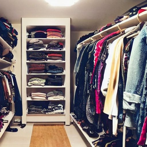
Alex proposes organizing your clothes into an endless, boundlessly wide, tall closet. Then, when you request a specific item, you only have to inform Alex of its position, and they will sew the piece from scratch using a reliable sewing machine. It soon dawns on you that arranging similar items close to one another is essential, allowing Alex to recreate them accurately based solely on their location.
After a few weeks of fine-tuning and adapting the closet’s arrangement, you and Alex establish a mutual understanding of its structure. Now, you can simply inform Alex of any clothing item’s location, and they can reproduce it impeccably!
This achievement makes you wonder: what if you provided Alex with an empty spot within the limitless closet? Astonishingly, Alex manages to create brand-new clothing items that never existed before! Although the process has imperfections, you now possess infinite possibilities for generating novel clothing. All it takes is selecting a space in the vast closet and allowing Alex to work wonders with the sewing machine.
With the story analogy in mind, let’s now develop a technical understanding of Autoencoders.
What Are Autoencoders?
An autoencoder is an artificial neural network used for unsupervised learning tasks (i.e., no class labels or labeled data) such as dimensionality reduction, feature extraction, and data compression. They seek to:
- Accept an input set of data (i.e., the input)
- Internally compress the input data into a latent space representation (i.e., a single vector that compresses and quantifies the input)
- Reconstruct the input data from this latent representation (i.e., the output)
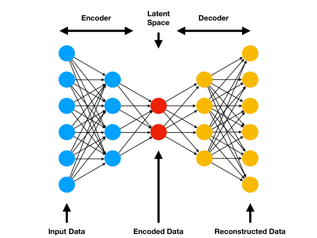
An autoencoder consists of the following two primary components:
- Encoder: The encoder compresses input data into a lower-dimensional representation known as the latent space or code. This latent space, often called embedding, aims to retain as much information as possible, allowing the decoder to reconstruct the data with high precision. If we denote our input data as
 and the encoder as
  , then the output latent space representation,
  , would be
 ") .
. - Decoder: The decoder reconstructs the original input data by accepting the latent space representation . If we denote the decoder function as
 and the output of the detector as
  , then we can represent the decoder as
 ") .
.
Both encoder and decoder are typically composed of one or more layers, which can be fully connected, convolutional, or recurrent, depending on the input data’s nature and the autoencoder’s architecture.
By using our mathematical notation, the entire training process of the autoencoder can be written as follows:
)")
Figure 2 demonstrates the basic architecture of an autoencoder:
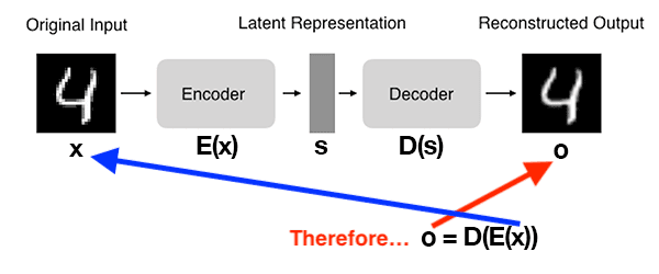
In this example, you can observe the following steps:
- We input a digit into the autoencoder.
- The encoder subnetwork generates a latent representation of the digit
4, which is considerably smaller in dimensionality than the input. - The decoder subnetwork reconstructs the original digit using the latent representation.
Therefore, you can think of an autoencoder as a network designed to reconstruct its input!
How Autoencoders Achieve High-Quality Reconstructions?
An autoencoder aims to reduce the discrepancy, or loss, between the original data and the reconstructed data at the decoder end, aiming to recreate the input as accurately as possible. This loss function is often referred to as the reconstruction error. The most common loss functions used for autoencoders are mean squared error (MSE) or binary cross-entropy (BCE), depending on the input data’s nature.
Revisiting the Story
With the story analogy fresh in our minds, let’s connect it to the technical concept of Autoencoders. In the story, you act as the encoder, organizing each clothing item into a specific location within the wardrobe and assigning an encoding. Meanwhile, your friend Alex takes on the role of the decoder, selecting a location in the wardrobe and attempting to recreate (or, in technical terms) the clothing item (a process referred to as decoding).
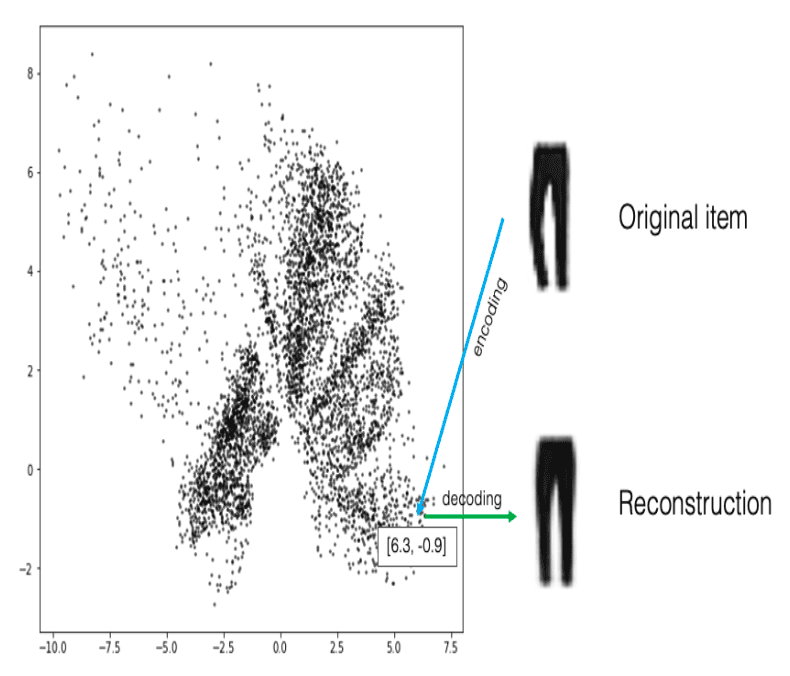
Figure 3 illustrates the visualization of the latent space and the process we discussed in the story, which aligns with the technical definition of the encoder and decoder. In the figure below, you encode the trouser by placing it in a specific location within the infinite closet (in a 2D space). Alex then reconstructs the item using the same or a very similar location.
Types of Autoencoder
There are several types of autoencoders, each with its unique properties and use cases.
Vanilla Autoencoder
Figure 4 shows the simplest form of an autoencoder, consisting of one or more fully connected layers for both the encoder and decoder. It works well for simple data but may struggle with complex patterns.
Convolutional Autoencoder (CAE)
Utilizes convolutional layers in both the encoder and decoder, making it suitable for handling image data. By exploiting the spatial information in images, CAEs can capture complex patterns and structures more effectively than vanilla autoencoders and accomplish tasks such as image segmentation, as shown in Figure 5.
![Figure 5: Architecture of Convolutional Autoencoder for Image Segmentation (source: Bandyopadhyay, “Autoencoders in Deep Learning: Tutorial & Use Cases [2023],” V7Labs, 2023).](https://pyimagesearch.com/wp-content/uploads/2023/07/conv-AE.png)
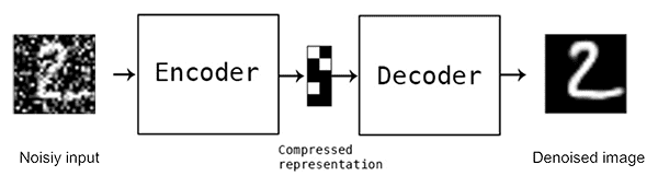
Denoising Autoencoder
This autoencoder is designed to remove noise from corrupted input data, as shown in Figure 6. During training, the input data is intentionally corrupted by adding noise, while the target remains the original, uncorrupted data. The autoencoder learns to reconstruct the clean data from the noisy input, making it useful for image denoising and data preprocessing tasks.
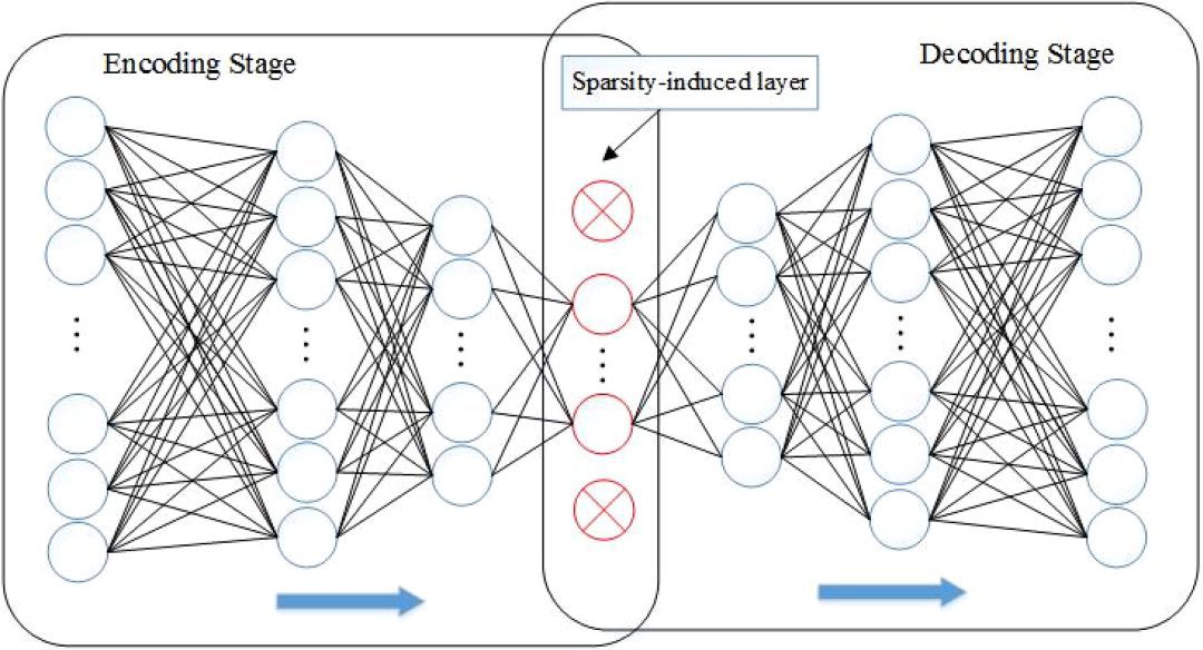
Sparse Autoencoder
This type of autoencoder enforces sparsity in the latent space representation by adding a sparsity constraint to the loss function (as shown in Figure 7). This constraint encourages the autoencoder to represent the input data using a small number of active neurons in the latent space, resulting in more efficient and robust feature extraction.
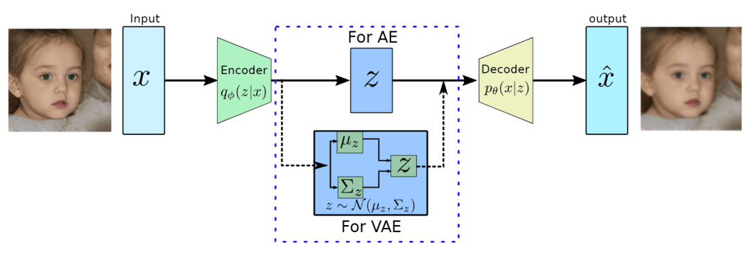
Variational Autoencoder (VAE)
Figure 8 shows a generative model that introduces a probabilistic layer in the latent space, allowing for sampling and generation of new data. VAEs can generate new samples from the learned latent distribution, making them ideal for image generation and style transfer tasks.
Sequence-to-Sequence Autoencoder
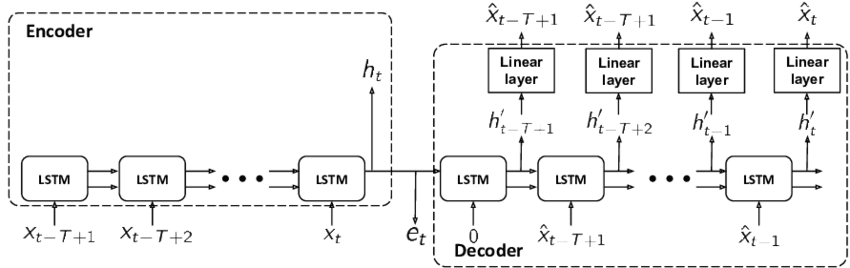
Also known as a Recurrent Autoencoder, this type of autoencoder utilizes recurrent neural network (RNN) layers (e.g., long short-term memory (LSTM) or gated recurrent unit (GRU)) in both the encoder and decoder shown in Figure 9. This architecture is well-suited for handling sequential data (e.g., time series or natural language processing tasks).
These are just a few examples of the various autoencoder architectures available. Each type is designed to address specific challenges and applications, and by understanding their unique properties, you can choose the most suitable autoencoder for your problem.
To implement an autoencoder in PyTorch, you would typically define two separate modules for the encoder and decoder, and then combine them in a higher-level module. You then train the autoencoder using backpropagation and gradient descent, minimizing the reconstruction error.
In summary, autoencoders are powerful neural networks with diverse applications in unsupervised learning, including dimensionality reduction, feature extraction, and data compression. By understanding their architecture, types, and implementation using frameworks like PyTorch, you can harness their capabilities to solve a wide range of real-world problems.
What Are the Applications of Autoencoders?
Autoencoders have a wide range of applications across various domains, including:
Dimensionality Reduction
Autoencoders can reduce the dimensionality of input data by learning a compact and efficient representation in the latent space. This can be helpful for visualization, data compression, and speeding up other machine learning algorithms.
Feature Learning
Autoencoders can learn meaningful features from input data, which can be used for downstream machine learning tasks like classification, clustering, or regression.
Anomaly Detection
By training an autoencoder on normal data instances, it can learn to reconstruct those instances with low error. When presented with an anomalous data point, the autoencoder will likely have a higher reconstruction error, which can be used to identify outliers or anomalies.
Denoising Images
Autoencoders can be trained to reconstruct clean input data from noisy versions. The denoising autoencoder learns to remove the noise and produce a clean version of the input data.
Image Inpainting
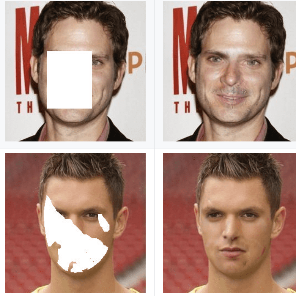
As shown in Figure 10, autoencoders can fill in missing or corrupted parts of an image by learning the underlying structure and patterns in the data.
Generative Modeling
Variational autoencoders (VAEs) and other generative variants can generate new, realistic data samples by learning the data distribution during training. This can be useful for data augmentation or creative applications.
Recommender Systems
Autoencoders can be used to learn latent representations of users and items in a recommender system, which can then predict user preferences and make personalized recommendations.
Sequence-to-Sequence Learning
Autoencoders can be used for sequence-to-sequence tasks, such as machine translation or text summarization, by adapting their architecture to handle sequential input and output data.
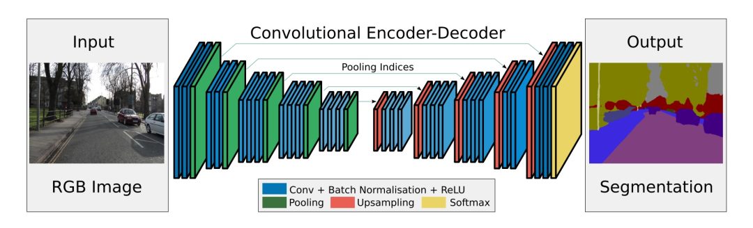
Image Segmentation
Autoencoders are commonly utilized in semantic segmentation as well. A notable example is SegNet (Figure 11), a model designed for pixel-wise, multi-class segmentation on urban road scene datasets. This model was created by researchers from the University of Cambridge’s Computer Vision Group.
These are just a few examples of the many possible applications of autoencoders. Their versatility and adaptability make them an important tool in the machine learning toolbox.
How Are Autoencoders Different from GANs?
For those familiar with Generative Adversarial Networks (GANs), you might wonder how Autoencoders, which also learn to generate images, differ from GANs. While both Autoencoders and GANs are generative models, they differ in architecture, training process, and objectives.
Architecture
- Autoencoders consist of an encoder and a decoder. The encoder compresses the input data into a lower-dimensional latent representation while the decoder reconstructs the input data from the latent representation.
- GANs consist of a generator and a discriminator. The generator creates fake samples from random noise, and the discriminator tries to differentiate between real samples from the dataset and fake samples produced by the generator.
Training Process
- Autoencoders are trained using a reconstruction error, which measures the difference between the input and reconstructed data. The training process aims to minimize this error.
- GANs use a two-player minimax game during training. The generator tries to produce samples that the discriminator cannot distinguish from real samples, while the discriminator tries to improve its ability to differentiate between real and fake samples. The training process involves finding an equilibrium between the two competing networks.
Objectives
- Autoencoders are primarily used for dimensionality reduction, data compression, denoising, and representation learning.
- GANs are primarily used for generating new, realistic samples, often in the domain of images, but also in other data types such as text, audio, and more.
While both autoencoders and GANs can generate new samples, they have different strengths and weaknesses. Autoencoders generally produce smoother and more continuous outputs, while GANs can generate more realistic and diverse examples but may suffer from issues like mode collapse. The choice between the two models depends on the specific problem and desired outcomes.
What’s next? I recommend PyImageSearch University.
78 total classes • 97+ hours of on-demand code walkthrough videos • Last updated: July 2023
★★★★★ 4.84 (128 Ratings) • 16,000+ Students Enrolled
I strongly believe that if you had the right teacher you could master computer vision and deep learning.
Do you think learning computer vision and deep learning has to be time-consuming, overwhelming, and complicated? Or has to involve complex mathematics and equations? Or requires a degree in computer science?
That’s not the case.
All you need to master computer vision and deep learning is for someone to explain things to you in simple, intuitive terms. And that’s exactly what I do. My mission is to change education and how complex Artificial Intelligence topics are taught.
If you’re serious about learning computer vision, your next stop should be PyImageSearch University, the most comprehensive computer vision, deep learning, and OpenCV course online today. Here you’ll learn how to successfully and confidently apply computer vision to your work, research, and projects. Join me in computer vision mastery.
Inside PyImageSearch University you’ll find:
- ✓ 78 courses on essential computer vision, deep learning, and OpenCV topics
- ✓ 78 Certificates of Completion
- ✓ 97+ hours of on-demand video
- ✓ Brand new courses released regularly, ensuring you can keep up with state-of-the-art techniques
- ✓ Pre-configured Jupyter Notebooks in Google Colab
- ✓ Run all code examples in your web browser — works on Windows, macOS, and Linux (no dev environment configuration required!)
- ✓ Access to centralized code repos for all 512+ tutorials on PyImageSearch
- ✓ Easy one-click downloads for code, datasets, pre-trained models, etc.
- ✓ Access on mobile, laptop, desktop, etc.
Summary
The blog post opens with an engaging story to help readers intuitively grasp the concept of autoencoders. It then defines autoencoders, explaining how they achieve high-quality reconstructions through their unique architecture. Revisiting the initial story, the concept of latent space, crucial to understanding autoencoders, is further unpacked.
Different types of autoencoders are then discussed, detailing their unique characteristics and functions. This leads to exploring the wide-ranging applications of autoencoders in various fields, such as image compression, denoising, and anomaly detection.
The post also differentiates between autoencoders and generative adversarial networks (GANs) by comparing their architecture, training process, and objectives.
In the upcoming tutorial, we will delve deeper and proceed to build a convolutional autoencoder with PyTorch, utilizing the Fashion-MNIST dataset. Furthermore, we will conduct a comprehensive post-training analysis of the autoencoder, including sampling data points from the latent space and reconstructing these sampled points into images.
Citation Information
Sharma, A. “Introduction to Autoencoders,” PyImageSearch, P. Chugh, A. R. Gosthipaty, S. Huot, K. Kidriavsteva, and R. Raha, eds., 2023, https://pyimg.co/ehnlf
@incollection{Sharma_2023_IntroAutoencoders,
  author = {Aditya Sharma},
  title = {Introduction to Autoencoders},
  booktitle = {PyImageSearch},
  editor = {Puneet Chugh and Aritra Roy Gosthipaty and Susan Huot and Kseniia Kidriavsteva and Ritwik Raha},
  year = {2023},
  url = {https://pyimg.co/ehnlf},
}
Unleash the potential of computer vision with Roboflow – Free!
- Step into the realm of the future by signing up or logging into your Roboflow account. Unlock a wealth of innovative dataset libraries and revolutionize your computer vision operations.
- Jumpstart your journey by choosing from our broad array of datasets, or benefit from PyimageSearch’s comprehensive library, crafted to cater to a wide range of requirements.
- Transfer your data to Roboflow in any of the 40+ compatible formats. Leverage cutting-edge model architectures for training, and deploy seamlessly across diverse platforms, including API, NVIDIA, browser, iOS, and beyond. Integrate our platform effortlessly with your applications or your favorite third-party tools.
- Equip yourself with the ability to train a potent computer vision model in a mere afternoon. With a few images, you can import data from any source via API, annotate images using our superior cloud-hosted tool, kickstart model training with a single click, and deploy the model via a hosted API endpoint. Tailor your process by opting for a code-centric approach, leveraging our intuitive, cloud-based UI, or combining both to fit your unique needs.
- Embark on your journey today with absolutely no credit card required. Step into the future with Roboflow.
Join the PyImageSearch Newsletter and Grab My FREE 17-page Resource Guide PDF
Enter your email address below to join the PyImageSearch Newsletter and download my FREE 17-page Resource Guide PDF on Computer Vision, OpenCV, and Deep Learning.
The post Introduction to Autoencoders appeared first on PyImageSearch.
Responses