Depth-Aware Object Insertion in Videos using Python

Depth-Aware Object Insertion in Videos Using Python

Instructions for placing 3D models in videos with a depth-aware method using Python

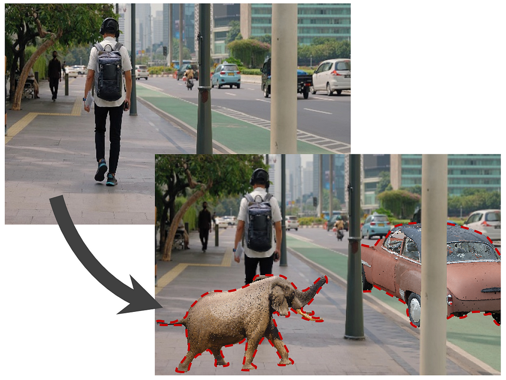
In the field of computer vision, the consistent estimation of depth and camera pose in videos has laid the foundation for more advanced operations, such as depth-aware object insertion in videos. Building on my previous article that explored these fundamental techniques, this article shifts focus toward depth-aware object insertion. Employing Python-based computational methods, I will outline a strategy for adding objects into pre-existing video frames in accordance with depth and camera orientation data. This methodology not only elevates the realism of edited video content but also has broad applications in video post-production.

In summary, the approach involves two main steps: first, estimating consistent depth and camera position in a video, and second, overlaying a mesh object onto the video frames. To make the object appear stationary in the 3D space of the video, it is moved in the opposite direction of any camera movement. This counter-movement ensures the object looks like it’s fixed in place throughout the video.

You can check my code on my GitHub page, which I will be referring to throughout this article.

Step 1: Generating camera pose matrices and consistent depth estimation of the video

In my previous article, I thoroughly explained how to estimate consistent depth frames of videos and the corresponding camera pose matrices throughout videos.

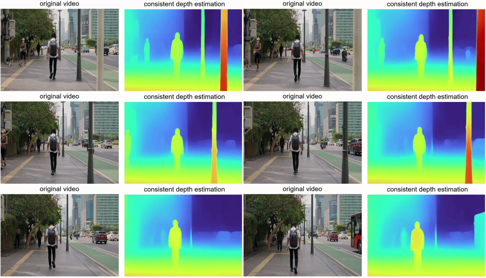
For this article, I selected a video featuring a man walking on a street, chosen specifically for its pronounced camera movement along an axis. This will allow for a clear evaluation of whether inserted objects maintain their fixed positions within the 3D space of the video.

I followed all the steps that I explained in my previous article to get the depth frames and the estimated camera pose matrices. We will especially need the “custom.matrices.txt” file generated by COLMAP.

Original footage and its estimated depth video are given below.

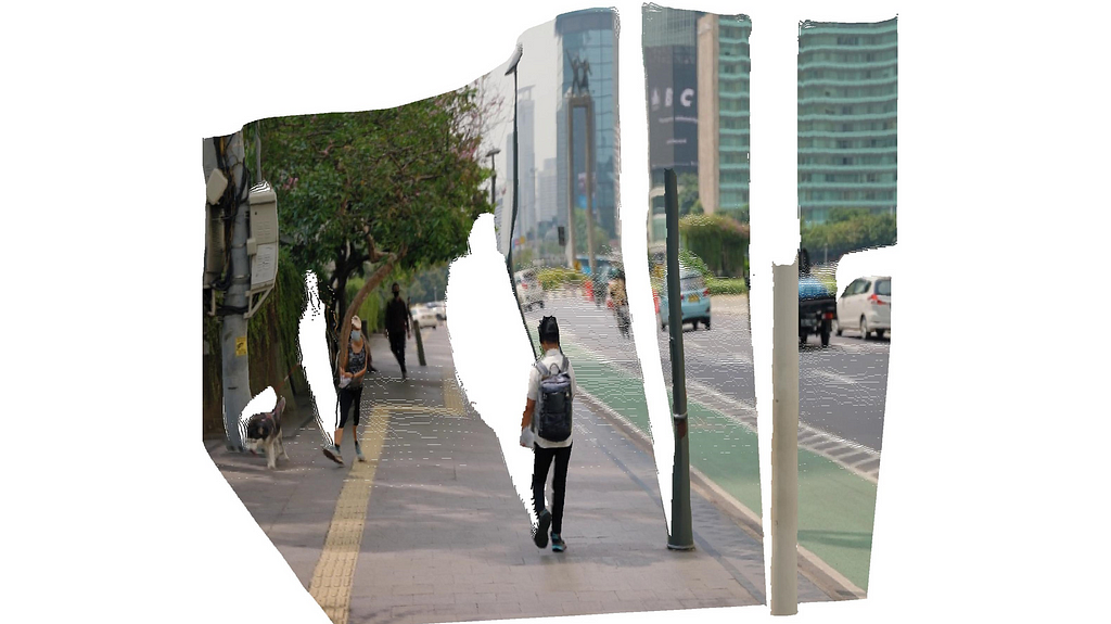
The point cloud visualization corresponding to the first frame is presented below. The white gaps indicate shadow regions that are obscured from the camera’s view due to the presence of foreground objects.

Step 2: Picking mesh files you want to insert

Now, we select the mesh files to be inserted into the video sequence. Various platforms such as Sketchfab.com and GrabCAD.com offer a wide range of 3D models to choose from.

For my demo video, I have chosen two 3D models, the links for which are provided in the image captions below:

I preprocessed the 3D models using CloudCompare, an open-source tool for 3D point cloud manipulation. Specifically, I removed the ground portions from the objects to enhance their integration into the video. While this step is optional, if you wish to modify certain aspects of your 3D model, CloudCompare comes highly recommended.

After pre-processing the mesh files, save them as .ply or .obj files. (Please note that not all 3D model file extensions support colored meshes, such as .stl).

Step 3: Re-rendering the frames with depth-aware object insertion

We now arrive at the core component of the project: video processing. In my repository, two key scripts are provided — video_processing_utils.py and depth_aware_object_insertion.py. As implied by their names, video_processing_utils.py houses all the essential functions for object insertion, while depth_aware_object_insertion.py serves as the primary script that executes these functions to each video frame within a loop.

A snipped version of the main section of depth_aware_object_insertion.py is given below. In a for loop that runs as many as the count of frames in the input video, we load batched information of the depth computation pipeline from which we get the original RGB frame and its depth estimation. Then we compute the inverse of the camera pose matrix. Afterwards, we feed the mesh, depth, and intrinsics of the camera into a function named render_mesh_with_depth().

for i in tqdm(range(batch_count)):

    batch = np.load(os.path.join(BATCH_DIRECTORY, file_names[i]))

    # ... (snipped for brevity)

    # transformation of the mesh with the inverse camera extrinsics
    frame_transformation = np.vstack(np.split(extrinsics_data[i],4))
    inverse_frame_transformation = np.empty((4, 4))
    inverse_frame_transformation[:3, :] = np.concatenate((np.linalg.inv(frame_transformation[:3,:3]),  
                                                          np.expand_dims(-1 * frame_transformation[:3,3],0).T), axi
    inverse_frame_transformation[3, :] = [0.00, 0.00, 0.00, 1.00]
    mesh.transform(inverse_frame_transformation)

    # ... (snipped for brevity)

    image = np.transpose(batch['img_1'], (2, 3, 1, 0))[:,:,:,0]    
    depth = np.transpose(batch['depth'], (2, 3, 1, 0))[:,:,0,0]

    # ... (snipped for brevity)

    # rendering the color and depth buffer of the transformed mesh in the image domain
    mesh_color_buffer, mesh_depth_buffer = render_mesh_with_depth(np.array(mesh.vertices), 
                                                                  np.array(mesh.vertex_colors), 
                                                                  np.array(mesh.triangles), 
                                                                  depth, intrinsics)
        
    # depth-aware overlaying of the mesh and the original image
    combined_frame, combined_depth = combine_frames(image, mesh_color_buffer, depth, mesh_depth_buffer) 

    # ... (snipped for brevity)

The render_mesh_with_depth function takes a 3D mesh, represented by its vertices, vertex colors, and triangles, and renders it onto a 2D depth frame. The function starts by initializing depth and color buffers to hold the rendered output. It then projects the 3D mesh vertices onto the 2D frame using camera intrinsic parameters. The function uses scanline rendering to loop through each triangle in the mesh, rasterizing it into pixels on the 2D frame. During this process, the function computes barycentric coordinates for each pixel to interpolate depth and color values. These interpolated values are then used to update the depth and color buffers, but only if the pixel’s interpolated depth is closer to the camera than the existing value in the depth buffer. Finally, the function returns the color and depth buffers as the rendered output, with the color buffer converted to a uint8 format suitable for image display.

def render_mesh_with_depth(mesh_vertices, vertex_colors, triangles, depth_frame, intrinsic):
    vertex_colors = np.asarray(vertex_colors)
    
    # Initialize depth and color buffers
    buffer_width, buffer_height = depth_frame.shape[1], depth_frame.shape[0]
    mesh_depth_buffer = np.ones((buffer_height, buffer_width)) * np.inf
    
    # Project 3D vertices to 2D image coordinates
    vertices_homogeneous = np.hstack((mesh_vertices, np.ones((mesh_vertices.shape[0], 1))))
    camera_coords = vertices_homogeneous.T[:-1,:]
    projected_vertices = intrinsic @ camera_coords
    projected_vertices /= projected_vertices[2, :]
    projected_vertices = projected_vertices[:2, :].T.astype(int)
    depths = camera_coords[2, :]

    mesh_color_buffer = np.zeros((buffer_height, buffer_width, 3), dtype=np.float32)
    
    # Loop through each triangle to render it
    for triangle in triangles:
        # Get 2D points and depths for the triangle vertices
        points_2d = np.array([projected_vertices[v] for v in triangle])
        triangle_depths = [depths[v] for v in triangle]
        colors = np.array([vertex_colors[v] for v in triangle])
        
        # Sort the vertices by their y-coordinates for scanline rendering
        order = np.argsort(points_2d[:, 1])
        points_2d = points_2d[order]
        triangle_depths = np.array(triangle_depths)[order]
        colors = colors[order]

        y_mid = points_2d[1, 1]

        for y in range(points_2d[0, 1], points_2d[2, 1] + 1):
            if y = buffer_height:
                continue
            
            # Determine start and end x-coordinates for the current scanline
            if y < y_mid:
                x_start = interpolate_values(y, points_2d[0, 1], points_2d[1, 1], points_2d[0, 0], points_2d[1, 0])
                x_end = interpolate_values(y, points_2d[0, 1], points_2d[2, 1], points_2d[0, 0], points_2d[2, 0])
            else:
                x_start = interpolate_values(y, points_2d[1, 1], points_2d[2, 1], points_2d[1, 0], points_2d[2, 0])
                x_end = interpolate_values(y, points_2d[0, 1], points_2d[2, 1], points_2d[0, 0], points_2d[2, 0])
            
            x_start, x_end = int(x_start), int(x_end)

            # Loop through each pixel in the scanline
            for x in range(x_start, x_end + 1):
                if x = buffer_width:
                    continue
                
                # Compute barycentric coordinates for the pixel
                s, t, u = compute_barycentric_coords(points_2d, x, y)
                
                # Check if the pixel lies inside the triangle
                if s >= 0 and t >= 0 and u >= 0:
                    # Interpolate depth and color for the pixel
                    depth_interp = s * triangle_depths[0] + t * triangle_depths[1] + u * triangle_depths[2]
                    color_interp = s * colors[0] + t * colors[1] + u * colors[2]
                    
                    # Update the pixel if it is closer to the camera
                    if depth_interp < mesh_depth_buffer[y, x]:
                        mesh_depth_buffer[y, x] = depth_interp
                        mesh_color_buffer[y, x] = color_interp

    # Convert float colors to uint8
    mesh_color_buffer = (mesh_color_buffer * 255).astype(np.uint8)
    
    return mesh_color_buffer, mesh_depth_buffer

Color and depth buffers of the transformed mesh are then fed into combine_frames() function along with the original RGB image and its estimated depthmap. This function is designed to merge two sets of image and depth frames. It uses depth information to decide which pixels in the original frame should be replaced by the corresponding pixels in the rendered mesh frame. Specifically, for each pixel, the function checks if the depth value of the rendered mesh is less than the depth value of the original scene. If it is, that pixel is considered to be “closer” to the camera in the rendered mesh frame, and the pixel values in both the color and depth frames are replaced accordingly. The function returns the combined color and depth frames, effectively overlaying the rendered mesh onto the original scene based on depth information.

# Combine the original and mesh-rendered frames based on depth information
def combine_frames(original_frame, rendered_mesh_img, original_depth_frame, mesh_depth_buffer):
    # Create a mask where the mesh is closer than the original depth
    mesh_mask = mesh_depth_buffer < original_depth_frame
    
    # Initialize combined frames
    combined_frame = original_frame.copy()
    combined_depth = original_depth_frame.copy()
    
    # Update the combined frames with mesh information where the mask is True
    combined_frame[mesh_mask] = rendered_mesh_img[mesh_mask]
    combined_depth[mesh_mask] = mesh_depth_buffer[mesh_mask]
    
    return combined_frame, combined_depth

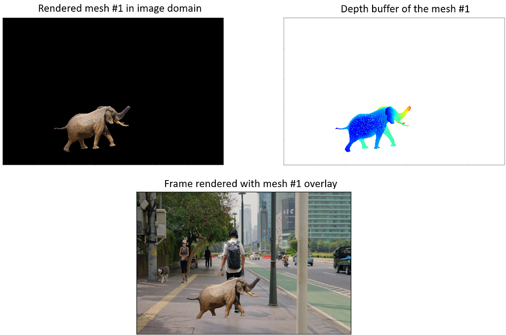
Here is how the mesh_color_buffer, mesh_depth_buffer and the combined_frame look like the first object, an elephant. Since the elephant object is not occluded by any other elements within the frame, it remains fully visible. In different placements, occlusion would occur.

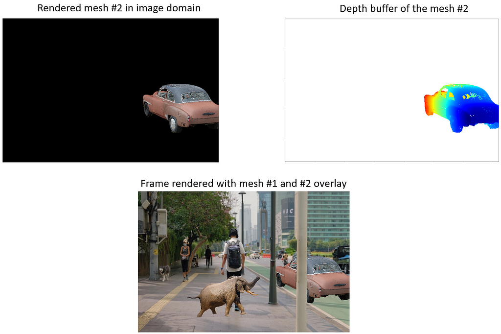
Accordingly, I placed the second mesh, the car, on the curbside of the road. I also adjusted its initial orientation such that it looks like it has been parked there. The following visuals are the corresponding mesh_color_buffer, mesh_depth_buffer and the combined_frame for this mesh.

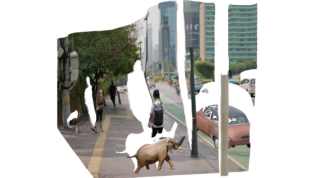
The point cloud visualization with both objects inserted is given below. More white gaps are introduced due to the new occlusion areas which came up with new objects.

After calculating the overlayed images for each one of the video frames, we are now ready to render our video.

Step 4: Rendering video from processed frames

In the last section of depth_aware_object_insertion.py, we simply render a video from the object-inserted frames using therender_video_from_frames function. You can also adjust the fps of the output video at this step. The code is given below:

video_name = 'depth_aware_object_insertion_demo.mp4'
save_directory = "depth_aware_object_insertion_demo/"
frame_directory = "depth_aware_object_insertion_demo/"
image_extension = ".png"
fps = 15 

# rendering a video of the overlayed frames
render_video_from_frames(frame_directory, image_extension, save_directory, video_name, fps)

Here is my demo video:

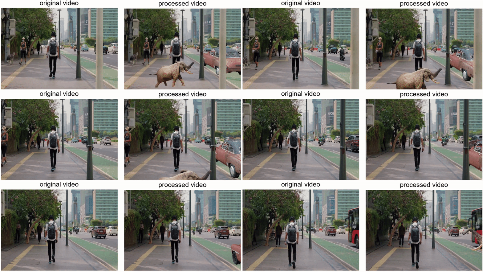
A higher-resolution version of this animation is uploaded to YouTube.

Overall, the object integrity appears to be well-maintained; for instance, the car object is convincingly occluded by the streetlight pole in the scene. While there is a slight perceptible jitter in the car’s position throughout the video —most likely due to imperfections in the camera pose estimation — the world-locking mechanism generally performs as expected in the demonstration video.

While the concept of object insertion in videos is far from novel, with established tools like After Effects offering feature-tracking-based methods, these traditional approaches often can be very challenging and costly for those unfamiliar with video editing tools. This is where the promise of Python-based algorithms comes into play. Leveraging machine learning and basic programming constructs, these algorithms have the potential to democratize advanced video editing tasks, making them accessible even to individuals with limited experience in the field. Thus, as technology continues to evolve, I anticipate that software-based approaches will serve as powerful enablers, leveling the playing field and opening up new avenues for creative expression in video editing.

Have a great day ahead!

Depth-Aware Object Insertion in Videos using Python was originally published in Towards Data Science on Medium, where people are continuing the conversation by highlighting and responding to this story.