DETR Breakdown Part 3: Architecture and Details

Table of Contents

DETR Breakdown Part 3: Architecture and Details

In this tutorial, we’ll learn about the model and architecture of DETR.

This lesson is the last of a 3-part series on DETR Breakdown:

1. DETR Breakdown Part 1: Introduction to DEtection TRansformers
2. DETR Breakdown Part 2: Methodologies and Algorithms
3. DETR Breakdown Part 3: Architecture and Details (this tutorial)

To learn about the model and architecture of Detection Transformers, just keep reading.

DETR Breakdown Part 3: Architecture and Details

We are at the final junction of our quest. In the first blog post of this series, we understood why and how DETR was born, its key features, and how it differs from previous models. In the previous blog post of this series, we looked at some methodologies used in DETR, specifically Set Prediction Loss.

This tutorial will examine the model to understand how each component comes together to achieve end-to-end object detection.

DETR Architecture 🏗️

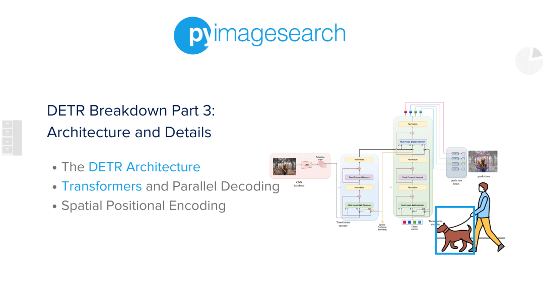
As is custom, we begin with a holistic overview of the entire DETR architecture as presented in this interactive diagram. Our goal would be to go through this tutorial and relate the explanations to each part of the diagram.

As we saw in the interactive diagram above, the entire DETR architecture consists of three main components:

1. CNN Backbone: To Extract a Compact Feature Representation
2. Transformer: The Encoder and Decoder Transformer
3. Feed-Forward Network: To Make the Final Detection Prediction

CNN Backbone 🦴

As shown in Figure 1, the CNN backbone is needed in DETR (Detection Transformer) because it serves as a feature extractor responsible for converting input images into a compact yet informative representation that the subsequent transformer architecture can use for object detection and localization tasks. In addition, CNNs are also inherently good at capturing spatial relationships within images, which is immensely beneficial for object detection tasks.

Starting with the input image , which has 3 color channels, the authors employ a standard Convolutional Neural Network (CNN) to create a lower-resolution activation map. The input and output tensors on the CNN Backbone with their shape are shown in Figure 2.

The reduced-resolution activation map serves as the extracted feature set generated by the CNN. This feature map, denoted as , possesses the following dimensions:

• The number of channels () is 2048,
• The height () is reduced by a factor of 32 from the original height (),
• The width () is similarly reduced by a factor of 32 from the original width ().

In essence, the feature map retains significant information from the input image while substantially reducing its spatial dimensions, thus facilitating further processing and analysis.

This enables the transformer architecture in DETR to focus on learning to detect and localize objects effectively.

Transformer Preprocessing ⚙️

Now that we have extracted the image features, the feature map is ready to be fed into the transformer encoder.

However, transformer encoders are designed to process sequences of tokens, which means the tensor representing the feature map must undergo further processing before it can be passed to the encoder.

When looking at the feature map’s shape, it’s obvious that we need extra steps to make it work well with the transformer encoder.

To do this, we first apply a 1×1 convolution to the high-level feature map, as shown in Figure 3. This helps us reduce the size of the channels from a larger number, , to a smaller one, .

This step is important because it makes the process more efficient and saves resources for the next steps. As a result, we created a new feature map called .

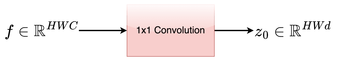
However, the feature map still cannot be directly passed into the transformer encoder due to its 2D spatial structure. Therefore, the feature map undergoes an additional reshaping step after the 1×1 convolution to resolve this issue.

In this step, the spatial dimensions are collapsed into a single dimension, effectively transforming the 2D feature map into a sequence of tokens suitable for input to the transformer encoder.

Transformer Encoder 🔄

ENCODER: Now that the feature map is reshaped into a sequence of tokens, we can send it over to the encoder. The Encoder is highlighted in Figure 4. Each layer within the encoder follows a standard architecture comprising two main components:

1. Multi-head self-attention module
2. Feed-forward neural network (FFN)

The transformer architecture doesn’t naturally pay attention to the order of the input elements. This means it doesn’t automatically understand the position or sequence of the input tokens. To fix this issue and ensure that the position information is included properly, we add special position-related information called fixed spatial positional encodings to the input of each attention layer. This helps the transformer understand the order and position of the elements in the input.

Transformer Decoder 🔄

This model’s decoder (shown in Figure 5) is based on a common structure used in transformers. It works with smaller pieces of information, each having a size of , and uses a method called multi-headed self-attention. Unlike the first-ever transformer design, this model doesn’t create the output one step at a time(autoregressive). Instead, it processes objects simultaneously in every decoder layer.

As the decoder is also permutation-invariant, meaning it doesn’t inherently account for the order of input tokens, the input embeddings must be distinct to produce different results. These input embeddings are learned positional encodings, referred to as object queries.

Wait a minute, what are Object Queries: In DETR, object queries play a key role in identifying and locating objects within an image. They act like “questions” that the model asks to find different objects in the image. Using object queries, the model can figure out where objects are, what they look like, and how many there are, all simultaneously, making the detection process more efficient and accurate.

Similar to the encoder, these object queries are added to the input of each attention layer. The decoder then transforms the object queries into output embeddings, which are subsequently decoded into box coordinates and class labels by a feed-forward network (explained in the following subsection). This process results in final predictions.

Prediction Heads: Feed-Forward Network ➡️🧠

The final prediction is calculated using a 3-layer perceptron (see Figure 6), a type of neural network with a ReLU (Rectified Linear Unit) activation function and a hidden dimension of size d.

A linear projection layer accompanies this FFN. The feed-forward neural network (FFN) predicts the bounding box’s normalized center coordinates, height, and width with respect to the input image. Meanwhile, the linear layer predicts the class label using a softmax function, which helps determine the most probable category for each object.

Since the model predicts a fixed-size set of bounding boxes, and is typically much larger than the actual number of objects of interest in an image, an additional special class label is used to represent that no object is detected within a particular slot.

This class is similar to the “background” class found in conventional object detection approaches, serving to identify regions of the image that do not contain any objects of interest.

Importance of DETR 🌟

🔁 End-to-End Trainability

One of the most significant advantages of DETR is its end-to-end trainability.

• DETR, unlike many traditional object detection models, does not rely on multiple stages of training and frequent manual adjustments.
• DETR streamlines the process by allowing for the simultaneous training of all components.
• This simplifies the overall workflow and helps to ensure more consistent performance across different datasets and scenarios.

⏩ Parallel Decoding for Enhanced Efficiency

DETR incorporates parallel decoding, which enables the model to process multiple objects simultaneously at each decoder layer.

• This improves the overall efficiency of the architecture.
• And also allows for better utilization of computational resources.
• By decoding objects in parallel, DETR can handle complex scenes with numerous objects more effectively than sequential decoding methods.

❌ Elimination of Hand-Crafted Features

Traditional object detectors often rely on hand-crafted features and region proposals.

• This can be time-consuming and challenging to develop.
• DETR, on the other hand, employs a more holistic approach that eliminates the need for these manual interventions.

🔎 Superior Attention Span with Transformers

Using transformers in DETR allows for a more efficient and flexible attention mechanism compared to conventional convolutional neural networks (CNNs).

• Transformers can effectively model long-range dependencies and capture complex relationships between objects in an image.
• This ability to focus on the most relevant parts of the input data leads to improved performance and more accurate object detection results.

🎯 Hungarian Matching and Set Prediction Loss

DETR incorporates Hungarian matching, which models the problem as a bipartite graph.

• This approach enables the model to consider all possible object permutations and effectively match predicted objects with ground truth labels.
• Using this bipartite matching loss function, DETR can better handle cases with multiple objects and varying numbers of objects in different images.

What’s next? I recommend PyImageSearch University.

Course information:
78 total classes • 97+ hours of on-demand code walkthrough videos • Last updated: July 2023
★★★★★ 4.84 (128 Ratings) • 16,000+ Students Enrolled

I strongly believe that if you had the right teacher you could master computer vision and deep learning.

Do you think learning computer vision and deep learning has to be time-consuming, overwhelming, and complicated? Or has to involve complex mathematics and equations? Or requires a degree in computer science?

That’s not the case.

All you need to master computer vision and deep learning is for someone to explain things to you in simple, intuitive terms. And that’s exactly what I do. My mission is to change education and how complex Artificial Intelligence topics are taught.

If you’re serious about learning computer vision, your next stop should be PyImageSearch University, the most comprehensive computer vision, deep learning, and OpenCV course online today. Here you’ll learn how to successfully and confidently apply computer vision to your work, research, and projects. Join me in computer vision mastery.

Inside PyImageSearch University you’ll find:

• ✓ 78 courses on essential computer vision, deep learning, and OpenCV topics
• ✓ 78 Certificates of Completion
• ✓ 97+ hours of on-demand video
• ✓ Brand new courses released regularly, ensuring you can keep up with state-of-the-art techniques
• ✓ Pre-configured Jupyter Notebooks in Google Colab
• ✓ Run all code examples in your web browser — works on Windows, macOS, and Linux (no dev environment configuration required!)
• ✓ Access to centralized code repos for all 512+ tutorials on PyImageSearch
• ✓ Easy one-click downloads for code, datasets, pre-trained models, etc.
• ✓ Access on mobile, laptop, desktop, etc.

Click here to join PyImageSearch University

Summary

In this tutorial on DEtection TRansformers (Architecture and Details), we unraveled the various components of this innovative framework that have changed the object detection landscape.

• We started with a broad overview of the DETR architecture, establishing a foundational understanding of the system.
• We then examined the Convolutional Neural Network (CNN) backbone, which processes raw images into image features.
• Our exploration continued with the preprocessing layer, a crucial element that ensured the compatibility of tensor shapes and sizes with the Transformer Encoder’s requirements.
• We then delved into the inner workings of the Encoder itself, highlighting DETR’s unique use of spatial positional encodings.
• Next, we looked at the Decoder, a significant component for understanding learned spatial embeddings or object queries.
• As we moved closer to the culmination of the architecture, we shed light on the prediction heads, or Feed-Forward Neural (FFN) layers, which output predictions.

Finally, we considered DETR’s importance in today’s world, recognizing the new ideas it’s brought forward and how it’s changed the way we do object detection.

Do you want us to cover the implementation of DETR in TensorFlow and Keras? Connect with us on Twitter by tagging @pyimagesearch.

Citation Information

A. R. Gosthipaty and R. Raha. “DETR Breakdown Part 3: Architecture and Details,” PyImageSearch, P. Chugh, S. Huot, K. Kidriavsteva, and A. Thanki, eds., 2023, https://pyimg.co/8depa

@incollection{ARG-RR_2023_DETR-breakdown-part3,
  author = {Aritra Roy Gosthipaty and Ritwik Raha},
  title = {{DETR} Breakdown Part 3: Architecture and Details},
  booktitle = {PyImageSearch},
  editor = {Puneet Chugh and Susan Huot and Kseniia Kidriavsteva and Abhishek Thanki},
  year = {2023},
  url = {https://pyimg.co/8depa},
}

Unleash the potential of computer vision with Roboflow – Free!

• Step into the realm of the future by signing up or logging into your Roboflow account. Unlock a wealth of innovative dataset libraries and revolutionize your computer vision operations.
• Jumpstart your journey by choosing from our broad array of datasets, or benefit from PyimageSearch’s comprehensive library, crafted to cater to a wide range of requirements.
• Transfer your data to Roboflow in any of the 40+ compatible formats. Leverage cutting-edge model architectures for training, and deploy seamlessly across diverse platforms, including API, NVIDIA, browser, iOS, and beyond. Integrate our platform effortlessly with your applications or your favorite third-party tools.
• Equip yourself with the ability to train a potent computer vision model in a mere afternoon. With a few images, you can import data from any source via API, annotate images using our superior cloud-hosted tool, kickstart model training with a single click, and deploy the model via a hosted API endpoint. Tailor your process by opting for a code-centric approach, leveraging our intuitive, cloud-based UI, or combining both to fit your unique needs.
• Embark on your journey today with absolutely no credit card required. Step into the future with Roboflow.

Join Roboflow Now

Join the PyImageSearch Newsletter and Grab My FREE 17-page Resource Guide PDF

Enter your email address below to join the PyImageSearch Newsletter and download my FREE 17-page Resource Guide PDF on Computer Vision, OpenCV, and Deep Learning.

Join the Newsletter!

Website

The post DETR Breakdown Part 3: Architecture and Details appeared first on PyImageSearch.